Chapter 10 Leptonic interactions

In this section we will study the electromagnetic and weak interactions involving the 3 generations of leptons.

10.1 Electromagnetic interactions

Background 10.1.1 (Feynman diagrams).

A convenient way to represent particle interactions are by Feynman diagrams. Associated with them are a set of Feynman rules, which are derived from quantum field theory and enable the calculation of the probability for each interaction to occur. We shall avoid the mathematical details, but use diagrams to understand the main features of the interactions.

The basic electromagnetic interactions where an electron either emits or absorbs a photon are

e^{-}\rightarrow e^{-}+\gamma\,,\quad\quad e^{-}+\gamma\rightarrow e^{-}\,.

(10.1)

These are represented by the diagrams in Fig. 10.1, where by convention time runs from left-to-right. The corresponding positron processes are also shown in Fig. 10.1. In this case, time again runs from left-to-right, but by convention an arrow pointing to the right represents a particle and an arrow pointing to the left represents an anti-particle.

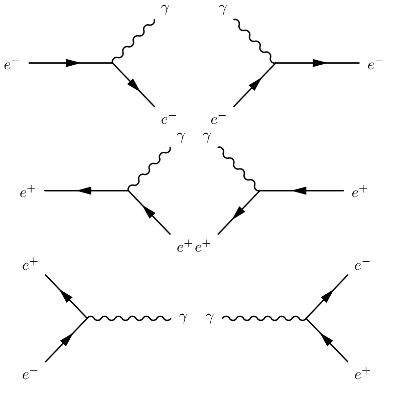
Six Feynman diagrams illustrate fundamental electron-photon interactions: electron and positron scattering, and pair production/annihilation. — Figure 10.1: (Top-left) $e^{-}\rightarrow e^{-}+\gamma$ ; (Top-right) $e^{-}+\gamma\rightarrow e^{-}$ ; (Middle-left) $e^{+}\rightarrow e^{+}+\gamma$ ; (Middle-right) $e^{+}+\gamma\rightarrow e^{+}$ ; (Bottom-left) $e^{+}+e^{-}\rightarrow\gamma$ ; (Bottom-right) $\gamma\rightarrow e^{+}+e^{-}$ .

Three Feynman diagrams showing leptons (electron, muon, and tau) absorbing or emitting a photon (gamma). — Figure 10.2: The basic vertex summarising the processes in Fig. 10.1. We also show this vertex for other charged leptons.

Notice that the arrows are continuous, which ensures charge (and lepton number, see later) conservation at the vertex. In Fig. 10.1 we also show the diagrams for $e^{+}e^{-}$ annihilation and creation.

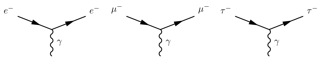
All these diagrams can conveniently be summarised by the vertex in Fig. 10.2, in which we also show the interactions of photons with other charged leptons.

Three Feynman diagrams show electron-electron scattering ($e^-e^- \to e^-e^-$) via the exchange of a virtual photon ($\gamma$) in the t-channel (left), u-channel (middle), and a superposition of the two (right). — Figure 10.3: $e^{-}+e^{-}\rightarrow e^{-}+e^{-}$ . The two diagrams with different time-orderings (left 2) are usually shown as one diagram (right) with the time-orderings implied.

10.1.1 Virtual Particles

Momentum is conserved at each vertex. However, it is easy to see energy conservation is violated for diagrams with a single vertex. We use $(E,{\bf p})$ to denote energy and momentum, which satisfy the relativistic relationship between energy and momentum Eqn. (13.3).

Consider the process (choosing the rest frame of the initial electron for simplicity)

e^{-}(E_{0},0)\rightarrow e^{-}(E_{p},{\bf-p})+\gamma(pc,\bf{p})

(10.2)

where $E_{0}=mc^{2}$ and $E_{p}=\sqrt{p^{2}c^{2}+m^{2}c^{4}}$ . It is easy to see by calculating $\Delta E=E_{p}+pc-E_{0}$ that energy is violated for all finite momenta $p$ .

This is why these processes are called virtual, as they cannot occur in isolation in free space. For a real process, we need at least two vertices combined in such a way that energy is only violated for a short time in accordance with the uncertainty principle. Incoming and outgoing free particles satisfy the relation Eqn. (13.3), but the virtual particles do not.

A simplified Feynman diagram shows an electron-electron scattering interaction with two intermediate photons. — Figure 10.4: $e^{-}+e^{-}\rightarrow e^{-}+e^{-}$ with two-photon exchange.

Example 10.1.1 (Range of Force).

Calculate the range of the exchange force for the following process in the low momenta limit.

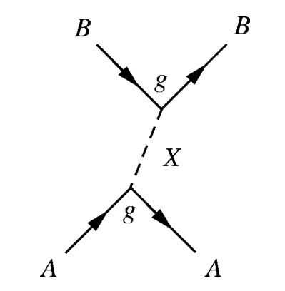
A t-channel Feynman diagram shows two particles A scattering into two particles B via the exchange of a dashed line particle X, with coupling g at both vertices.

Solution.

In the rest frame of particle A the lower vertex represents

A(E_{0},0)\rightarrow A(E_{A},{\bf-p})+X(E_{X},{\bf p})

(10.3)

where $E_{0}=m_{A}c^{2}$ , $E_{A}=\sqrt{p^{2}c^{2}+m_{A}^{2}c^{4}}$ and $E_{X}=\sqrt{p^{2}c^{2}+m_{X}^{2}c^{4}}$ . The change in energy is

\Delta E=\sqrt{p^{2}c^{2}+m_{A}^{2}c^{4}}+\sqrt{p^{2}c^{2}+m_{X}^{2}c^{4}}-m_{% A}c^{2}\,.

(10.4)

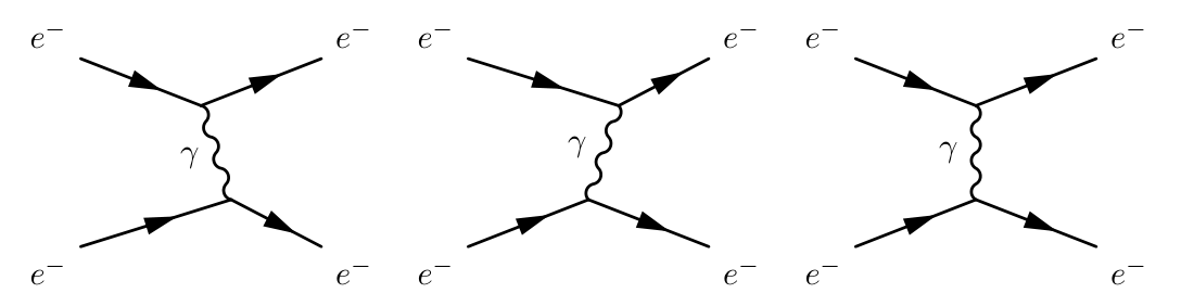
In the limit $p\rightarrow 0$ this is $\Delta E=m_{X}c^{2}$ . Using the uncertainty relation $\Delta t\sim\hbar/\Delta E$ and $R\sim c\Delta t$ then $R\sim\hbar/(m_{X}c)$ .

For example, the scattering process

e^{-}+e^{-}\rightarrow e^{-}+e^{-}\,,

(10.5)

shown in Fig. 10.3 has two vertices and the exchange of a single photon. This is called the lowest-order diagram. You can keep adding more vertices to make more complex diagrams with more than one exchange photon, but these are lower amplitude processes.

10.1.2 Time ordering

Note that for Fig. 10.3 there are two ways of time-ordering the photon exchange (i.e. whether the upper initial electron emits or absorbs the virtual photon). Normally we draw one diagram, as shown in the bottom panel of Fig. 10.3, with the different time-orderings implied.

However is it crucial to remember these when actually calculating the probability amplitude of a process – they all contribute. You should also be careful with this when there is the exchange of charged $W^{\pm}$ , since the particular time-ordering will fix the charge.

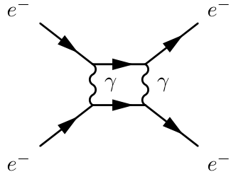
10.1.3 Higher order diagrams

We can also draw more complicated diagrams, for example including two-photon exchange, as shown in Fig. 10.4 (question: how many time-orderings are there?). However, from quantum field theory, it is shown that each photon vertex contributes a probability of $\alpha$ to the scattering process, where the fine structure constant is

\alpha=\frac{e^{2}}{4\pi\epsilon_{0}\hbar c}\approx\frac{1}{137}\,.

(10.6)

Higher-order photon exchange is therefore suppressed.

10.2 Leptons and the weak interaction

Recall that the six leptons appear in 3 generations,

\left(\begin{array}[]{c}\nu_{e}\\ e^{-}\end{array}\right)\,,\quad\left(\begin{array}[]{c}\nu_{\mu}\\ \mu^{-}\end{array}\right)\,,\quad\left(\begin{array}[]{c}\nu_{\tau}\\ \tau^{-}\end{array}\right)\,.

Each generation of lepton has an associated conservation law. Electron lepton number is defined as

L_{\rm e}=N(e^{-})-N(e^{+})+N(\nu_{e})-N(\bar{\nu}_{e})\,.

(10.7)

Here the notation $e^{\pm}$ denotes an anti-electron or positron. $N(e^{+})$ is the number of positrons, $N(e^{-})$ is the number of electrons, $N(\nu_{e})$ is the number of electron neutrinos and $N(\bar{\nu}_{e})$ the number of electron anti-neutrinos. It is found experimentally that, during the course of the interaction, the quantity $L_{\rm e}$ is constant which is conserved in the interaction. There must be a symmetry which gives rise to this conservation law. Muon lepton number is defined similarly as

L_{\mu}=N(\mu^{-})-N(\mu^{+})+N(\nu_{\mu})-N(\bar{\nu}_{\mu})\,,

(10.8)

and the tau lepton number

L_{\tau}=N(\tau^{-})-N(\tau^{+})+N(\nu_{\tau})-N(\bar{\nu}_{\tau})

(10.9)

The three quantum numbers $L_{\rm e},L_{\mu}$ , and $L_{\tau}$ are conserved in the standard model. How can we test to see if there are processes in which these laws are violated? We need to find a process that violates these laws. An example is

\mu^{-}\rightarrow e^{-}+e^{+}+e^{-}

(10.10)

This process could occur on energy grounds since $m_{\mu}=105.7\,{\rm MeV/c}^{2}$ and $m_{\rm e}=0.511\,{\rm MeV/c}^{2}$ . There is lots of energy, much more than is needed, but the process has never been seen.

The statement can be made more precise. We define the branching ratio as the probability that a process occurs in the decay of a particle. The probability that a muon decays into two electrons and a positron is found experimentally by measuring the fraction of such decays that occur out of the total number of decay events. Thus

P=\frac{N(\mu^{-}\rightarrow e^{-}+e^{+}+e^{-})}{N(\mu^{-}\rightarrow{\rm all% \,\,products})}

(10.11)

In $10^{12}$ decays no $\mu^{-}\rightarrow e^{-}+e^{+}+e^{-}$ decays have been seen, so we can say the branching ratio is less than $10^{-12}$ . It could be much less than this and finite; it could be zero (since the decay violates the conservation of $L_{\rm e}$ and $L_{\mu}$ ).

10.2.1 Leptonic weak interactions

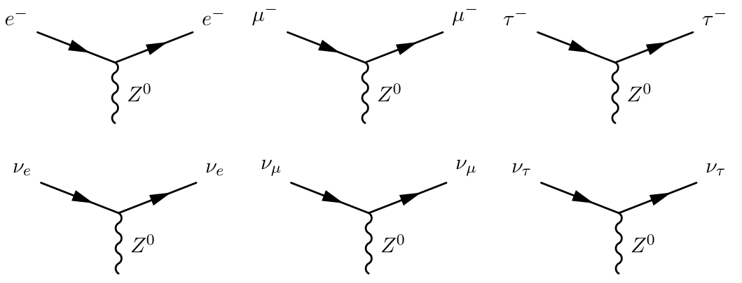
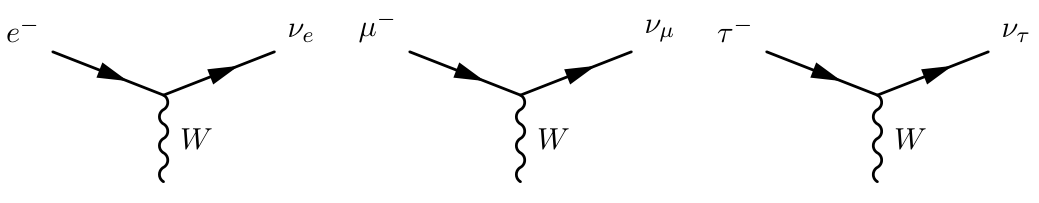
For the moment we focus on purely leptonic interactions. Weak interactions involving leptons are represented by exchange processes in which a $W^{\pm}$ or $Z^{0}$ is emitted by one lepton and absorbed by another. In analogy with the electromagnetic case discussed above, the basic vertices for $Z^{0}$ interactions are shown in Fig. 10.5. Notice that charge and lepton number are conserved at each vertex. The basic vertices for $W^{\pm}$ interactions are shown in Fig. 10.6. Charge and lepton number is also conserved. One should assign the correct charge to the $W^{\pm}$ under the understanding that it is either emitted or absorbed.

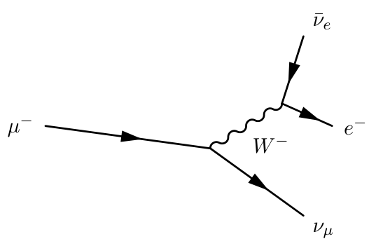
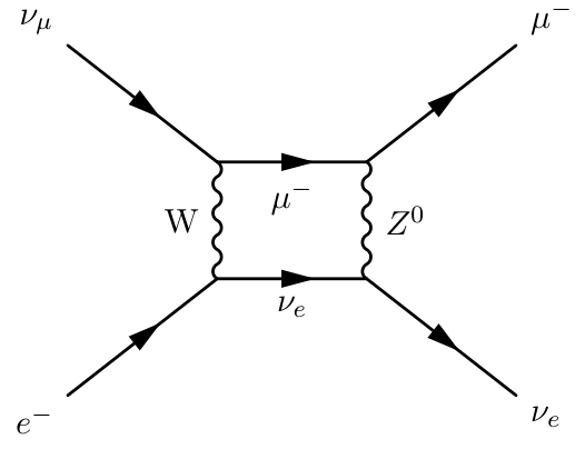
Six Feynman diagrams illustrate neutral current interactions involving leptons and the Z boson: three charged lepton interactions ($e^-$, $\mu^-$, $\tau^-$) and three neutrino interactions ($\nu_e$, $\nu_\mu$, $\nu_\tau$). — Figure 10.5: The basic vertices summarising $Z^{0}$ exchange.

Three Feynman diagrams depict leptonic weak interaction vertices where an incoming charged lepton interacts with a W boson to produce a corresponding neutrino. — Figure 10.6: The basic vertices summarising $W^{\pm}$ exchange.

As an example consider muon decay. The dominant diagram is shown in Fig. 10.7. As with the electromagnetic interaction higher order processes are possible. A diagram for inverse muon decay, for example, is shown in Fig. 10.8. Detailed calculation, however, again shows these higher-order diagrams are highly suppressed.

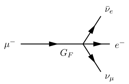
At low energies, the de Broglie wavelengths of the incoming and outgoing particles are much larger than the range of the $W^{\pm}$ exchange. In this case we can approximate the diagram by a zero-range point interaction, as shown in Fig. 10.9. The strength of the interaction is characterised by the Fermi coupling constant, $G_{F}$ ,

\frac{G_{F}}{\left(\hbar c\right)^{3}}=1.166\times 10^{-5}\,{\rm GeV}^{-2}\,.

(10.12)

The relation between the coupling constant and the mass of the exchange particle $M_{W}$ is

\frac{G_{F}}{\sqrt{2}\left(\hbar c\right)^{3}}=\frac{4\pi\alpha_{W}}{\left(M_{% W}c^{2}\right)^{2}}\,,

(10.13)

where $\alpha_{W}$ is a dimensionless parameter in analogy with the fine structure constant.

A Feynman diagram showing muon decay ($\mu^-$) into a muon neutrino ($\nu_\mu$) and a W boson ($W^-$), which then decays into an electron ($e^-$) and an electron antineutrino ($\bar{\nu}_e$). — Figure 10.7: Dominant diagram for muon decay.

A Feynman diagram illustrating a weak interaction process, likely $\nu_\mu + e^- \to \mu^- + \nu_e$, via a box diagram with an intermediate $W$ and $Z^0$ boson exchange. — Figure 10.8: Example of higher order inverse muon decay.

A Feynman diagram of muon decay ($\mu^- \rightarrow e^- + \bar{\nu}_e + \nu_{\mu}$) via a four-fermion interaction labeled $G_F$. — Figure 10.9: Inverse muon decay and the zero range approximation.

10.3 Exercises

Example 10.3.1.

For each of the following decays state a conservation law that forbids it

1.

$n\rightarrow p+e^{-}$
2.

$n\rightarrow\pi^{+}+e^{-}$
3.

$n\rightarrow p+\pi^{-}$
4.

$n\rightarrow p+\gamma$

Solution.

1.

Conservation of electron lepton number $L_{e}$ violated.
2.

Conservation of electron lepton number $L_{e}$ and baryon number $B$ violated.
3.

This satisfies conservation of baryon number and charge, however the rest mass energy of a neutron only exceeds that of a proton by about 1 MeV. The rest mass energy of a pion is substantially more than this (around 100 MeV) so the conservation of energy is violated.
4.

Conservation of electric charge is violated.